Home » Free Excel Tips » Custom Fill Series

Excel Fill Series and Pick From Custom List

Custom Excel Fill Series

How many times have you typed Jan, Feb, Mar in a column? Do you create lots of charts for each plant or hospital in your company? If you are typing the same thing over and over again, there is a better (and much faster) way!

Let's say you need to create a column with Jan-05 to Dec-05. Here is how Excel's custom fill series works.

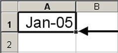
• Type Jan 2005 in a cell.
• Now click on the cell and notice that the lower right corner has a box:
  
  

• Click on the box and drag it down 11 rows.
• Presto - you now have column with Jan-05 to Dec-05:
  
  

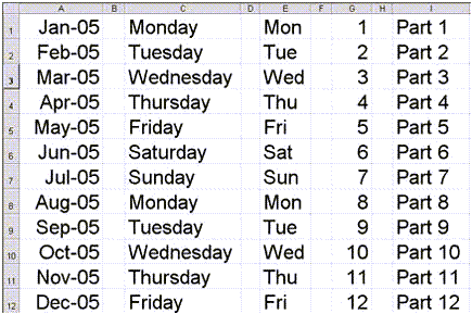
Pretty simple isn't it? Drag the box down 23 rows and get Jan-05 to Dec-06. Try this with Monday thru Friday, 1, 2, 3 or Part 1, Part 2, etc.

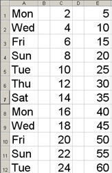
You can also create a pattern and Excel will follow it. Type in cell 1 and then in cell 2. Excel will detect a pattern and follow it. Here is an example of creating a column with every other day.

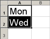
Select both cells and then grab the lower right box and drag down as many rows as you want. Use this to count by 2s, 5s, etc.

You can also create your own Excel custom list. Let's say you do lots of charts with the same five locations. Denver, Los Angeles, New York, Orlando, Phoenix. If you already have these cities typed in a spreadsheet do the following:

• Click and drag over the cells with the cities to select them
• Go to Tools/Options/Custom Lists and select Import then OK
• This will create an Excel custom list
• To access your new list, type the first value in the list (i.e. Denver), then select the cell with Denver in it and drag down the lower right box to the next four cells.

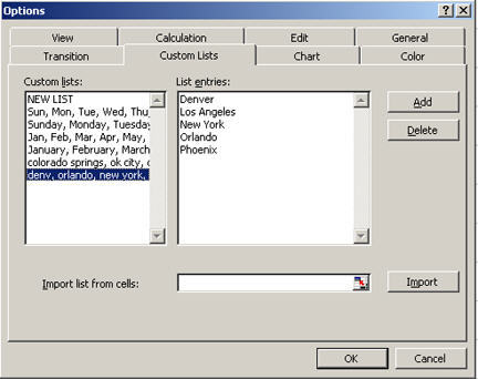
If you don't already have these values in a spreadsheet go to Tools/ Options/ Custom Lists and select Add. Type your list into the box. Then click on Add again to create the list. For more information on this functionality go to Excel's help index and type in Custom, Fill Series.

Excel Pick From List

Excels Pivot Table function can help you summarize large spreadsheets of raw data. Unfortunately, the Pivot Table requires values to be EXACTLY the same to summarize them. Do you know how many ways there are to spell Colorado Springs? (Colo Springs, CO Springs, Colo Sprgs, CO Sprgs, etc.) How about Accounts Payable? I am sure you have your own personal favorite.

When setting up a spreadsheet for others to populate, you can create a finite list of selections for them to use and then have them access the list using Excel's Pick From List function. Here's how:

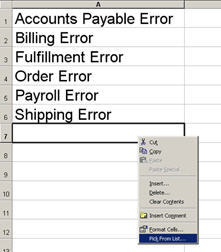
• Create your finite list of error codes, cities, etc. in a spreadsheet.
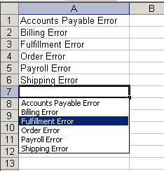
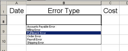
• Right click on the next cell under the list and select "Pick From List". Excel will bring a up a pull down of options from your list.
• Select one and the cell will be populated with that value.

You can show your master list or hide it. To hide it, select the rows with your list, then click on Format, Row, Hide.

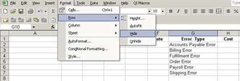
Right click on the cell below the hidden row to view and select from the pull down list:

Application for QI Macros

Use the Custom Fill Series to save time when creating your data sheets. Use the Excel Pick From List function to obtain consistent descriptions for fields that you want to total with Excels Pivot Table function and then create a Pareto or bar chart.

---

Stop using old technology!

Upgrade Your Excel and Data Analysis Skills to Smart Charts Using QI Macros.