Do You Struggle with Creating PivotTables in Excel?
QI Macros can create pivottables for you with one click!
No Other Software Can Do This!
Create PivotTables using QI Macros:
- Select 2-4 Column headings.
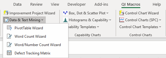
- Click on QI Macros menu > Data and Text Mining > PivotTable Wizard.
- QI Macros will analyze your data and format the PivotTable for you.
QI Macros Makes it Easy to Create PivotTables
If you are like many Excel users, you struggle with creating PivotTables in Excel. However, PivotTables are a valuable tool that every quality improvement professional should learn and know how to use. QI Macros makes creating PivotTables easy. Here is how.
- Perform some basic data cleanup on your "flat" transaction files like the one below:
- Make sure each column has a distinct heading.
- Check for misspellings or inconsistencies in your data. For example, Hosp1 and Hospital 1 will be treated as two different values by Excel. Use Excel's Find and Replace function to make these consistent.
- Next click on one to four columns of data to select them. These columns will be included in your PivotTable. In the example below, we selected four columns of data (region, entity, admit date, and charges).
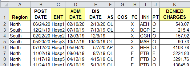
Above sample data found in Documents > QI Macros Test Data >
Improvement Project Wizard.xlsx (or datamining.xlsx) > "Healthcare Denied Claims" tab
- Next, click on the QI Macros menu, and select the PivotTable Wizard in the Data & Text Mining section:
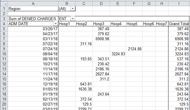
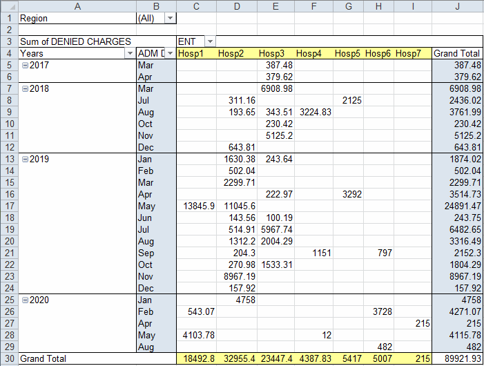
- Based on the frequency of values in each column, the QI Macros PivotTable Wizard figures out where to place each slice of data and automatically creates a PivotTable for you:
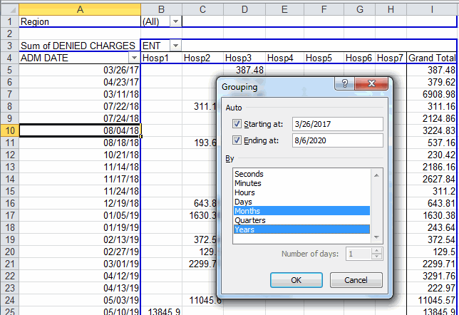
- These pivot tables can then be grouped by date or rearranged as required. To group dates, right click on any date, then select Group and define your criteria:
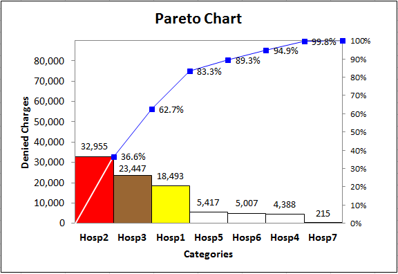
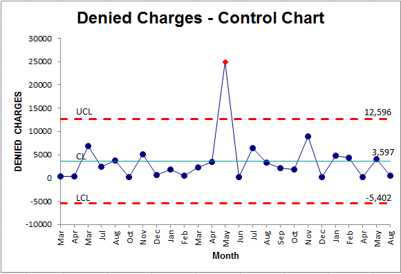
- Once you have the data view that makes sense, you can select data right from the PivotTable and draw charts using QI Macros. In the example below, select the cells highlighted in yellow to create a Pareto Chart and the cells highlighted in blue to create a control chart. Tip: Use the Ctrl-key to select non-adjacent columns. Also, note that the total in cell J30 is not selected:
NOTE: If your PivotTable output includes simply too much data, try selecting only (3) to (5) columns by focusing on:
- Date, Where, What, (How Much), (Who)?
Stop Struggling with PivotTables!
Start creating your PivotTables in just minutes.
Download a free 30-day trial. Get PivotTables now!
QI Macros Draws These Charts Too!