You Can Learn to Use Excel's Conditional Formatting
Conditional Formatting Has a Ton of Applications - here are a few
To Change the Color of the Bars on a Gantt Chart
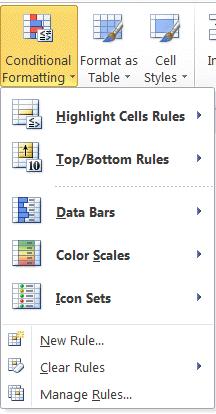
- Select "Manage Rules" under "Conditional Formatting," which is found under the "Home" tab in Excel:
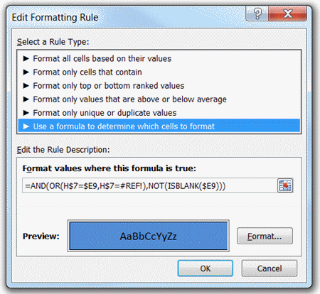
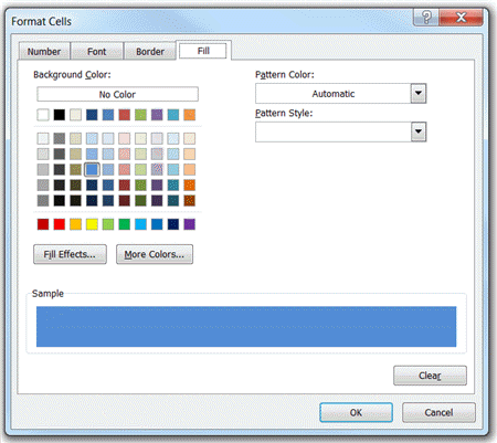
- Next, open the "Edit Formatting Rule" window and select "Format" and "Fill." Select your color, press "OK," then "Apply."
- Repeat this for all (3) rules found in the template.
 .
.
To Change the Color on Specific Parts of the Bar
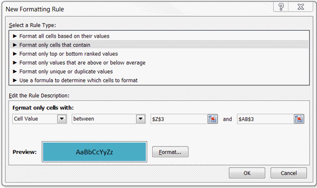
- Select the cells you wish to change the color of. Then, select "New Rule" under "Conditional Formatting"
- Next, open the "Edit Formatting Rule" window and select "Format only cells that contain." Then, select the cells you wish to change the color of, in "Format only cells with Cell Value between _ and _."
- Lastly, select your color through the "Format" button, press "OK," then "Apply.
Stop using old technology!
Upgrade Your Excel and Data Analysis Skills to Smart Charts Using QI Macros.
Track Data Over Time
Primitive Chart

Line Graph
Line Graph
Smart Chart
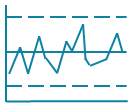
Control Chart
Control Chart
Compare Categories
Primitive Chart

Pie Chart
Pie Chart
Smart Chart

Pareto Chart
Pareto Chart
Analyze Variation
Primitive Chart
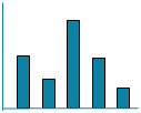
Bar or Column Chart
Bar or Column Chart
Smart Chart
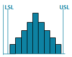
Histogram
Histogram
QI Macros add-in for Excel makes creating smart charts a snap.
Join 100,000+ Users
in 80 Countries