Merging Excel Worksheets or Workbooks
Using VLOOKUP, or OFFSET and MATCH Recently, I was working in Panama with a client implementing Lean Six Sigma. One of the participants had an unusual problem. She needed to integrate four different reports into one so that she could analyze several of their key process indicators (KPIs). Unfortunately, Excel doesn't provide an easy way to merge workbooks or worksheets based on a key. We could have exported the data into Access and merged them that way, but there's an easier way to do it right in Excel using VLOOKUP or OFFSET and MATCH functions.
Merge Excel Worksheets with VLOOKUP
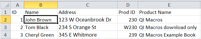
I've simplified the data to make the process easier to understand. It's pretty simple:- Put all of the worksheets to be merged into one workbook. The 3 worksheets in this example are named - Name, Address and Products.
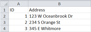
- Sort each worksheet in ascending order on its database "key". The key is the common field contained in each worksheet. In the Name and Address worksheets, the database key is the Record ID # in column A.
- In a new worksheet, enter the formulas to "look up" the database "key" in each worksheet.
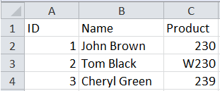
Name
Address
Products
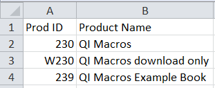
I want to merge name and address based on the common field "the ID", and then merge the product name in Products column B based on the product in the "name" worksheet column C.
I can use the VLOOKUP function to do this.
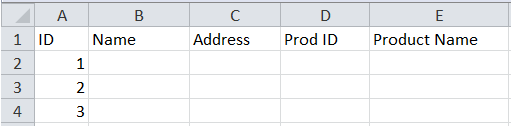
I start by creating a new worksheet and entering the headings in row 1 and the record IDs in column A. Then I put my cursor in cell B2 to build the VLOOKUP formula.
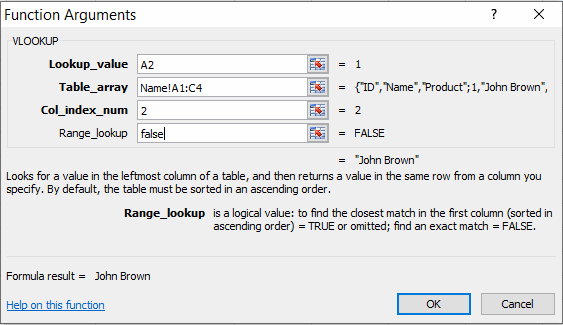
Click on the Insert function key and then find VLOOKUP under Lookup and Reference. Excel's function window will help you through this. Here is a brief explanation of each part of the formula:
- Lookup value - location of the value (the database key) I want to look up. Cell A2 in my example.
- Table Array - the worksheet and cells I want to look in to find the data I want to retrieve
- Col Index Num - the column in the Table Array that I want to get the data from.
- Range Lookup - select True for the closet match and False for an exact match.
Here is my final populated spreadsheet
The formulas to look up each field are:
- Customer name in the name worksheet: =VLOOKUP(A2,Name!A$1:C$4,2,TRUE)
- Customer address: =VLOOKUP(A2,Address!A$1:B$4,2,TRUE)
- Product Ordered: =VLOOKUP(A2,Name!A$1:C$4,3,TRUE)
- Product Name: =VLOOKUP(D2,Products!A$1:B$3,2,TRUE)
Merging Worksheets with OFFSET and MATCH
The process is the same except you don't have to sort the data:- Put all of the worksheets to be merged into one workbook.
- In a new worksheet, enter the formulas to "look up" the record IDs in each worksheet.
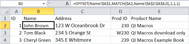
MATCH($A2,Name!$A$2:$A$4,0) will give us a "1" which is the first row of A2:A4.
OFFSET will use the index returned by MATCH to pick the correct field. For example:
OFFSET($A1,row,col,height,width) using 1 for row, 1 for col,1 for height, and 1 for width would offset from A1 by one row down, one column over for a height and width of one cell.
OFFSET ($A1,1,1,1,1) would select cell B2 (John Brown).
If we replace the "1" for the row with the MATCH formula (yes, you can "nest" formulas inside of other formulas), we get the desired merged cell:
The formulas to look up each field are:
- Customer name in the name worksheet:
=OFFSET(Name!$A$1,MATCH($A2,Name!$A$2:$A$4,0),1,1,1) - Customer address:
=OFFSET(Address!A$1,MATCH(A2,Address!A$2:A$4,0),1,1,1) - Product Ordered:
=OFFSET(Name!$A$1,MATCH($A2,Name!$A$2:$A$4,0),2,1,1) - Product Name:
=OFFSET(Products!$A$1,MATCH($D2,Products!$A$2:$A$4,0),1,1,1)
Download an Excel workbook with these worksheets and formulas.
Next Steps
Once all of the data is combined onto one worksheet, it becomes much easier to use pivot tables to summarize the data and create an improvement story using QI Macros.
Using VLOOKUP or OFFSET/MATCH isn't as easy as it could be, but it's a lot easier than trying to combine the data manually.
What data do you need to combine to perform a better, more detailed and robust analysis?
Stop using old technology!
Upgrade Your Excel and Data Analysis Skills to Smart Charts Using QI Macros.
Track Data Over Time
Line Graph
Control Chart
Compare Categories
Pie Chart
Pareto Chart
Analyze Variation
Bar or Column Chart
Histogram
QI Macros add-in for Excel makes creating smart charts a snap.
Join 100,000+ Users
in 80 Countries